| Study | \(p_0\) | \(p_1\) | \(a\) | \(b\) | \(c\) | \(d\) | \(RR\) | \(OR\) |
|---|---|---|---|---|---|---|---|---|
| A | 0.100 | 0.126 | 63 | 437 | 50 | 450 | 1.260 | 1.297 |
| B | 0.300 | 0.358 | 179 | 321 | 150 | 350 | 1.193 | 1.301 |
| C | 0.500 | 0.566 | 283 | 217 | 250 | 250 | 1.132 | 1.304 |
The previous posts built confidence intervals for the risk ratio of a single Brand Lift Study (BLS). This post addresses a different question: how to compare and aggregate effects across studies with different baseline response rates. The scale used to report a single campaign’s result to an advertiser and the scale used to pool results across studies serve different purposes and need not be the same.
The ceiling effect: RR and absolute lift depend on the baseline
\(RR = \frac{p_1}{p_0}\) is bounded above by \(\frac{1}{p_0}\), since \(p_1 \leq 1\). A study with \(p_0 = 0.50\) can produce at most \(RR = 2\). A study with \(p_0 = 0.05\) can produce at most \(RR = 20\). The maximum achievable \(RR\) is a property of the baseline, not of the ad’s effectiveness.
The absolute lift \(p_1 - p_0\) has the same problem in the other direction: its maximum is \(1 - p_0\). A study with \(p_0 = 0.80\) can produce at most \(p_1 - p_0 = 0.20\), regardless of how effective the ad is.
Both \(RR\) and absolute lift carry information about the baseline baked into their numerical value. Comparing \(RR = 1.30\) from one study to \(RR = 1.15\) from another and concluding the first ad was more effective requires the assumption that the two baselines impose similar constraints, which is rarely the case across BLS studies.
A baseline-free effect requires fixing a scale
Is there an effect measure that does not move with \(p_0\)? There is, but it requires choosing a scale on which the effect is defined to be constant. That choice is a model assumption.
The logistic regression model assumes ad exposure shifts the log-odds of a positive response by a constant \(\beta\):
\[\text{logit}(p_1) = \text{logit}(p_0) + \beta\]
Under this model, \(OR = \exp(\beta)\) is the same regardless of \(p_0\). Given \(p_0\) and \(OR\), the exposed rate is:
\[p_1 = \frac{p_0 \cdot OR}{1 - p_0 + p_0 \cdot OR}\]
Plugging in \(OR = 1.30\):
| \(p_0\) | \(p_1\) | \(RR\) | \(p_1 - p_0\) | \(OR\) |
|---|---|---|---|---|
| 0.05 | 0.064 | 1.278 | 0.014 | 1.30 |
| 0.10 | 0.126 | 1.262 | 0.026 | 1.30 |
| 0.30 | 0.358 | 1.193 | 0.058 | 1.30 |
| 0.50 | 0.565 | 1.130 | 0.065 | 1.30 |
\(OR\) is constant by construction. \(RR\) decreases from 1.278 to 1.130 as \(p_0\) increases: the ceiling compresses it. Absolute lift increases from 0.014 to 0.065. The same logit-scale effect produces different \(RR\) and \(p_1 - p_0\) values at different baselines.
This is a model assumption, not a fact. Whether ad exposure truly operates on the logit scale is untestable from a single 2×2 table. The assumption is adopted because it makes cross-study comparison coherent, not because it is known to be correct.
The odds ratio and the variance of log(OR)
The odds ratio is defined as:
\[OR = \frac{p_1 / (1 - p_1)}{p_0 / (1 - p_0)}\]
Label the four cells of the 2×2 table as \(a = x_1\), \(b = n_1 - x_1\), \(c = x_0\), \(d = n_0 - x_0\). Then:
\[\widehat{OR} = \frac{a \cdot d}{b \cdot c}\]
\[\log(\widehat{OR}) = \text{logit}(\hat{p}_1) - \text{logit}(\hat{p}_0)\]
Apply the delta method to \(g(p) = \text{logit}(p) = \log(p) - \log(1-p)\). The derivative is \(g'(p) = \frac{1}{p(1-p)}\), so:
\[\text{Var}(\text{logit}(\hat{p})) \approx \frac{1}{[p(1-p)]^2} \cdot \frac{p(1-p)}{n} = \frac{1}{n \, p(1-p)}\]
Rewriting with cell counts \(x = np\) and \(n - x = n(1-p)\):
\[\text{Var}(\text{logit}(\hat{p})) = \frac{1}{x} + \frac{1}{n - x}\]
Since \(\hat{p}_1\) and \(\hat{p}_0\) are independent, the variance of the difference is the sum:
\[\text{Var}(\log(\widehat{OR})) = \frac{1}{a} + \frac{1}{b} + \frac{1}{c} + \frac{1}{d}\]
The first post derived \(\text{Var}(\log(\widehat{RR})) = \frac{1}{x_1} - \frac{1}{n_1} + \frac{1}{x_0} - \frac{1}{n_0}\), which can be rewritten as \(\frac{1}{a} - \frac{1}{a+b} + \frac{1}{c} - \frac{1}{c+d}\). The variance of \(\log(\widehat{OR})\) has a simpler form: four reciprocals with no subtraction.
Constructing the confidence interval for OR
The CI for \(\log(OR)\) follows the same structure as the log-transform CI for \(RR\) from the first post: symmetric on the log scale, exponentiated back.
\[\log(\widehat{OR}) \pm z_{1-\alpha/2} \times \sqrt{\frac{1}{a} + \frac{1}{b} + \frac{1}{c} + \frac{1}{d}}\]
Exponentiating:
\[\left( \widehat{OR} \cdot \exp(-z_{1-\alpha/2} \cdot SE), \quad \widehat{OR} \cdot \exp(+z_{1-\alpha/2} \cdot SE) \right)\]
where \(SE = \sqrt{\frac{1}{a} + \frac{1}{b} + \frac{1}{c} + \frac{1}{d}}\).
The interval is always positive, asymmetric around \(\widehat{OR}\), and equivariant under inversion of the table.
Two properties that distinguish log(OR) from log(RR)
Both \(\log(\widehat{RR})\) and \(\log(\widehat{OR})\) have closed-form variance formulas derived from the delta method. Both support log-transform CIs, SQL implementation, and inverse-variance weighting. The closed-form variance is not a differentiator. Two properties are.
Baseline independence under logit additivity. If ad exposure shifts log-odds by a constant \(\beta\), then \(OR = \exp(\beta)\) does not depend on \(p_0\). \(RR\) and \(p_1 - p_0\) do. This is the reason to use \(\log(OR)\) for cross-study aggregation: pooling \(\log(OR)\) values from studies with different baselines estimates a common effect on the logit scale. Pooling \(\log(RR)\) values conflates the ad effect with the baseline.
Transpose symmetry. Swapping rows (exposed \(\leftrightarrow\) control) or columns (positive \(\leftrightarrow\) negative) in the 2×2 table maps \(\log(OR) \to -\log(OR)\): the sign flips, the magnitude is unchanged. \(\text{Var}(\log(\widehat{OR})) = \frac{1}{a} + \frac{1}{b} + \frac{1}{c} + \frac{1}{d}\) is symmetric in all four cells, reflecting this property. \(\text{Var}(\log(\widehat{RR})) = \frac{1}{a} - \frac{1}{a+b} + \frac{1}{c} - \frac{1}{c+d}\) is not symmetric: swapping positive and negative produces a different variance, because \(RR\) does not have transpose symmetry.
When the odds ratio approximates the risk ratio
The two measures are related by an identity:
\[OR = RR \times \frac{1 - p_0}{1 - p_1}\]
When both \(p_0\) and \(p_1\) are small, \(\frac{1 - p_0}{1 - p_1} \approx 1\) and \(OR \approx RR\).
BLS baselines are not small. Typical values range from 10% to 40%. At these levels, \(OR\) and \(RR\) diverge:
| \(p_0\) | \(p_1\) | \(RR\) | \(OR\) |
|---|---|---|---|
| 0.02 | 0.024 | 1.200 | 1.205 |
| 0.10 | 0.120 | 1.200 | 1.227 |
| 0.30 | 0.360 | 1.200 | 1.313 |
At \(p_0 = 0.30\) with \(RR = 1.20\), the \(OR\) is \(1.31\), a 55% overstatement of the lift if misread as a risk ratio. In BLS contexts, \(OR\) must not be interpreted as lift. The reporting scale for advertisers remains \(RR - 1\) (relative lift) or \(p_1 - p_0\) (absolute lift). \(\log(OR)\) serves a different purpose: aggregation.
Worked example: three studies at different baselines
Fix \(\beta = \log(1.30) = 0.2624\) and construct three synthetic studies with \(n_1 = n_0 = 500\). Cell counts are \(n \times p\) rounded to the nearest integer.
The log-odds effect is the same across all three studies by construction. \(RR\) ranges from 1.132 (study C, \(p_0 = 0.50\)) to 1.260 (study A, \(p_0 = 0.10\)). Ranking by \(RR\) would make study A appear most effective. Ranking by \(OR\) gives approximately the same value for all three.
The per-study CIs for \(OR\):
| Study | \(\log(\widehat{OR})\) | \(SE^2\) | \(SE\) | CI lower | CI upper |
|---|---|---|---|---|---|
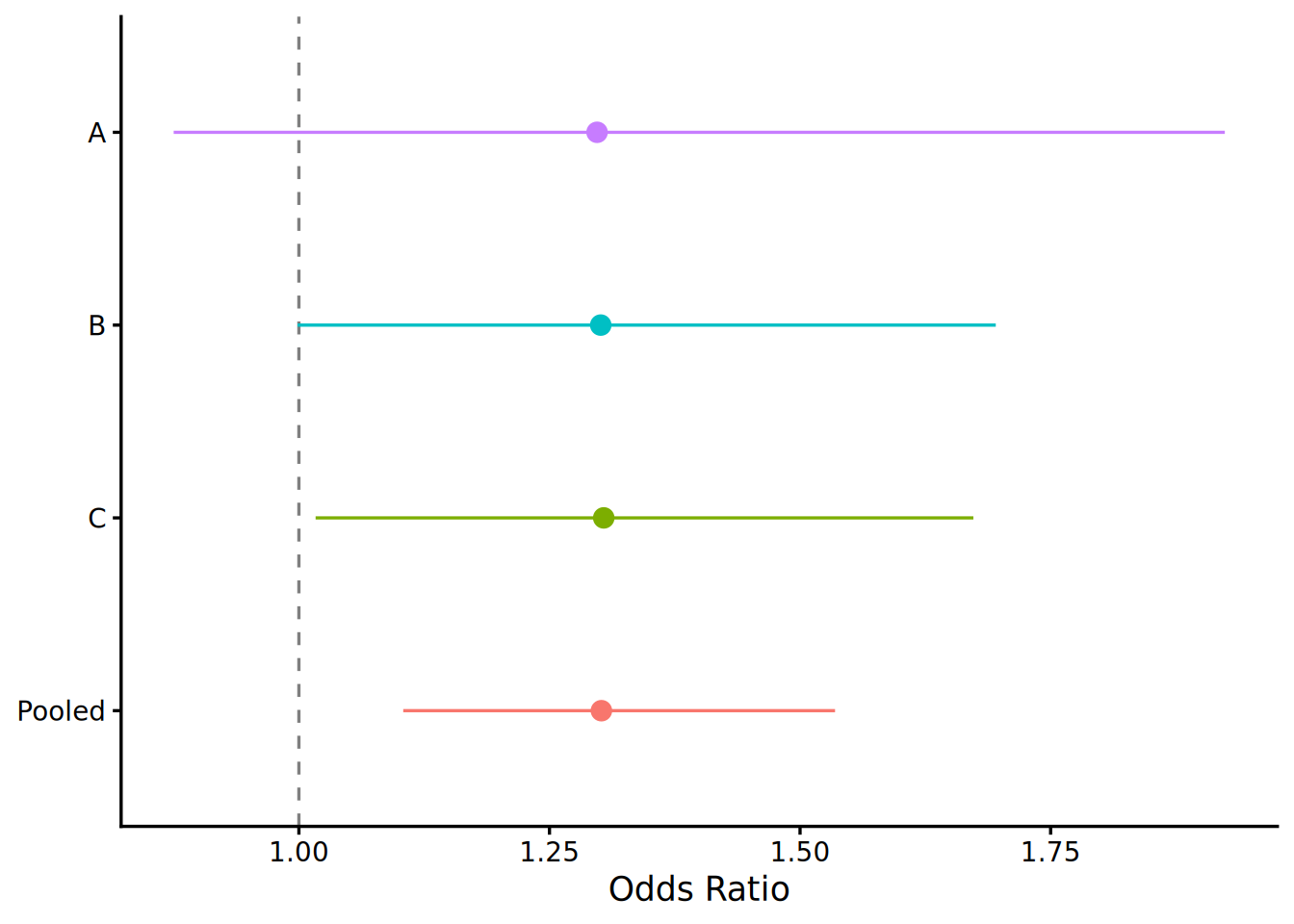
| A | 0.2604 | 0.0404 | 0.2010 | 0.875 | 1.924 |
| B | 0.2632 | 0.0182 | 0.1350 | 0.999 | 1.695 |
| C | 0.2655 | 0.0161 | 0.1271 | 1.017 | 1.673 |
Study A has the widest CI (\(SE = 0.201\)), driven by the small control positive count \(c = 50\): the \(\frac{1}{c}\) term dominates. Study C has the narrowest (\(SE = 0.127\)), because all four cells are large. Only study C’s CI excludes \(1\) at the 95% level.
Aggregation: why not merge the tables?
The three 2×2 tables could be summed cell-by-cell into a single pooled table. If the \(OR\) is the same within each study, the pooled \(OR\) should recover that common value. It does not. A numerical example with two studies, each with \(OR = 4.0\) and \(n_1 = n_0 = 1{,}000\):
| Study | \(p_0\) | \(p_1\) | \(OR\) |
|---|---|---|---|
| A | 0.100 | 0.308 | 4.000 |
| B | 0.400 | 0.727 | 4.000 |
| Merged | 0.250 | 0.517 | 3.217 |
Both studies have \(OR = 4.0\), but the merged table gives \(OR = 3.22\). Summing the tables distorts the \(OR\), even though the within-study effect is the same. (\(RR\) does not have this problem: merging preserves a common \(RR\).) The fix is straightforward: compute \(\log(\widehat{OR})\) within each study, then pool the estimates.
Pooling study-level log(OR)
The inverse-variance weighted mean of \(\log(\widehat{OR})\) across \(K\) studies is:
\[\log(\widehat{OR})_{\text{pooled}} = \frac{\sum_{k=1}^{K} w_k \log(\widehat{OR}_k)}{\sum_{k=1}^{K} w_k}\]
where \(w_k = \frac{1}{\text{Var}(\log(\widehat{OR}_k))} = \frac{1}{\frac{1}{a_k} + \frac{1}{b_k} + \frac{1}{c_k} + \frac{1}{d_k}}\).
The variance of the pooled estimate is \(\text{Var}(\log(\widehat{OR})_{\text{pooled}}) = \frac{1}{\sum_{k} w_k}\), and the 95% CI is:
\[\log(\widehat{OR})_{\text{pooled}} \pm 1.96 \times \frac{1}{\sqrt{\sum_k w_k}}\]
Worked example: pooling the three studies
| Study | \(\log(\widehat{OR})\) | \(SE^2\) | \(w\) | \(w \times \log(\widehat{OR})\) |
|---|---|---|---|---|
| A | 0.2604 | 0.0404 | 24.7625 | 6.4488 |
| B | 0.2632 | 0.0182 | 54.8677 | 14.4435 |
| C | 0.2655 | 0.0161 | 61.9507 | 16.4510 |
\[\sum w_k = 141.58, \quad \log(\widehat{OR})_{\text{pooled}} = \frac{37.3433}{141.58} = 0.2638\]
\[SE_{\text{pooled}} = \frac{1}{\sqrt{141.58}} = 0.0840\]
\[\text{95\% CI for } \log(OR): \quad 0.2638 \pm 1.96 \times 0.0840 = (0.0990, \; 0.4285)\]
\[\text{95\% CI for } OR: \quad (e^{0.0990}, \; e^{0.4285}) = (1.104, \; 1.535)\]
None of the three individual studies produced a CI that cleanly excluded \(1\) at the 95% level (only study C barely did). The pooled CI excludes \(1\), with a lower bound above \(1.1\). Aggregation recovered the signal that the individual studies could not establish alone.
Study C receives the largest weight (\(w_C\)) because its four cells are all large, producing the smallest variance. Study A receives the smallest weight: its control positive count \(c = 50\) inflates the \(\frac{1}{c}\) term. The weights automatically downweight less precise estimates, without any manual judgment about which studies to include.