Every Brand Lift Study (BLS) is a 2×2 table: exposed vs. control, positive response vs. not. The risk ratio \(RR = \frac{p_1}{p_0}\), where \(p_1\) and \(p_0\) are the positive response rates in the exposed and control groups, is the most direct measure of how much exposure shifted the outcome. An \(RR\) of \(1.12\) means the exposed group responded positively 12% more often than control. Platforms typically report \(RR - 1\) as “relative lift”, but the underlying quantity is a ratio of two binomial proportions.
No major ad platform constructs a confidence interval for \(RR\) that accounts for the sampling variability in both \(p_1\) and \(p_0\). Google Ads and DV360 build CIs on absolute lift \((p_1 - p_0)\): 80% two-sided for Google Ads, 90% for DV360. Both define relative lift as absolute lift divided by \(p_0\). The reported relative lift CI is consistent with dividing the absolute lift CI endpoints by \(p_0\), treating it as a known constant (Andrews 2020). Meta uses a Bayesian framework and reports posterior probability rather than a frequentist CI. In all cases, the uncertainty in \(p_0\) is ignored. The result is a CI that is too narrow.
The difficulty in building a proper CI for \(RR\) is that dividing one sample proportion by another produces a sampling distribution that is asymmetric, bounded below by zero, and has variance that depends on both \(p_1\) and \(p_0\) in a nonlinear way.
This post builds a confidence interval for \(RR\) using the delta method, step by step.
Setup
A BLS campaign produces the following data:
| Positive | Negative | Total | |
|---|---|---|---|
| Exposed | \(x_1\) | \(n_1 - x_1\) | \(n_1\) |
| Control | \(x_0\) | \(n_0 - x_0\) | \(n_0\) |
The positive response rates are:
\[\hat{p}_1 = \frac{x_1}{n_1}, \quad \hat{p}_0 = \frac{x_0}{n_0}\]
The risk ratio is:
\[\widehat{RR} = \frac{\hat{p}_1}{\hat{p}_0}\]
Each \(\hat{p}\) is a sample proportion from a binomial distribution. Their variances are:
\[\text{Var}(\hat{p}_1) = \frac{p_1(1 - p_1)}{n_1}, \quad \text{Var}(\hat{p}_0) = \frac{p_0(1 - p_0)}{n_0}\]
The exposed and control groups are independently randomized, so \(\hat{p}_1\) and \(\hat{p}_0\) are independent.
The naive approach: delta method directly on RR
The delta method says: if \(\hat{\theta}\) is an asymptotically normal estimator of \(\theta\), then for a differentiable function \(g\),
\[\text{Var}(g(\hat{\theta})) \approx \left[ g'(\theta) \right]^2 \text{Var}(\hat{\theta})\]
This comes from a first-order Taylor expansion of \(g\) around \(\theta\):
\[g(\hat{\theta}) \approx g(\theta) + g'(\theta)(\hat{\theta} - \theta)\]
The first term is a constant, so the variance of the right-hand side is \([g'(\theta)]^2 \, \text{Var}(\hat{\theta})\).
For a function of two variables \(g(p_1, p_0) = \frac{p_1}{p_0}\), the same logic extends. The first-order Taylor expansion around \((p_1, p_0)\) is:
\[g(\hat{p}_1, \hat{p}_0) \approx g(p_1, p_0) + \frac{\partial g}{\partial p_1}(\hat{p}_1 - p_1) + \frac{\partial g}{\partial p_0}(\hat{p}_0 - p_0)\]
The right-hand side, minus the constant \(g(p_1, p_0)\), is a linear combination \(aU + bV\) where \(a = \frac{\partial g}{\partial p_1}\), \(b = \frac{\partial g}{\partial p_0}\), \(U = \hat{p}_1 - p_1\), \(V = \hat{p}_0 - p_0\). The variance of a linear combination is:
\[\text{Var}(aU + bV) = a^2 \text{Var}(U) + b^2 \text{Var}(V) + 2ab\,\text{Cov}(U, V)\]
which gives:
\[\text{Var}(\widehat{RR}) \approx \left(\frac{\partial g}{\partial p_1}\right)^2 \text{Var}(\hat{p}_1) + \left(\frac{\partial g}{\partial p_0}\right)^2 \text{Var}(\hat{p}_0) + 2 \frac{\partial g}{\partial p_1} \frac{\partial g}{\partial p_0} \text{Cov}(\hat{p}_1, \hat{p}_0)\]
Since \(\hat{p}_1\) and \(\hat{p}_0\) are independent, \(\text{Cov}(\hat{p}_1, \hat{p}_0) = 0\) and the cross term vanishes:
\[\text{Var}(\widehat{RR}) \approx \left(\frac{\partial g}{\partial p_1}\right)^2 \text{Var}(\hat{p}_1) + \left(\frac{\partial g}{\partial p_0}\right)^2 \text{Var}(\hat{p}_0)\]
The partial derivatives are:
\[\frac{\partial}{\partial p_1}\left(\frac{p_1}{p_0}\right) = \frac{1}{p_0}, \quad \frac{\partial}{\partial p_0}\left(\frac{p_1}{p_0}\right) = -\frac{p_1}{p_0^2}\]
Substituting:
\[\text{Var}(\widehat{RR}) \approx \frac{1}{p_0^2} \cdot \frac{p_1(1-p_1)}{n_1} + \frac{p_1^2}{p_0^4} \cdot \frac{p_0(1-p_0)}{n_0}\]
which simplifies to:
\[\text{Var}(\widehat{RR}) \approx RR^2 \left[ \frac{1-p_1}{n_1 p_1} + \frac{1-p_0}{n_0 p_0} \right]\]
\(\hat{p}_1\) and \(\hat{p}_0\) are asymptotically normal by the central limit theorem. The delta method preserves asymptotic normality, so \(\widehat{RR}\) is also asymptotically normal. The standard Wald interval is:
\[\widehat{RR} \pm 1.96 \times \sqrt{\text{Var}(\widehat{RR})}\]
This is a valid first-order approximation, but it has a structural problem: the interval is symmetric around \(\widehat{RR}\). Since \(RR\) is bounded below by zero and has a right-skewed sampling distribution, a symmetric interval can:
- Produce a negative lower bound, which is impossible for a ratio of probabilities.
- Undercover on the right tail, where the true RR is more likely to lie when the point estimate is large.
Delta method on log(RR)
Applying the delta method to \(\log(RR)\) instead of \(RR\) directly solves both problems. \(\log\) maps \((0, \infty)\) to \((-\infty, \infty)\), so a symmetric interval on the log scale, when exponentiated back, produces an asymmetric interval on the original scale that can never go negative.
Write:
\[\log(\widehat{RR}) = \log(\hat{p}_1) - \log(\hat{p}_0)\]
Since \(\hat{p}_1\) and \(\hat{p}_0\) are independent, the variance of the difference is the sum of the variances:
\[\text{Var}(\log(\widehat{RR})) = \text{Var}(\log(\hat{p}_1)) + \text{Var}(\log(\hat{p}_0))\]
Apply the univariate delta method to each term. For \(g(p) = \log(p)\), \(g'(p) = 1/p\), so:
\[\text{Var}(\log(\hat{p}_1)) \approx \frac{1}{p_1^2} \cdot \frac{p_1(1 - p_1)}{n_1} = \frac{1 - p_1}{n_1 \, p_1}\]
\[\text{Var}(\log(\hat{p}_0)) \approx \frac{1}{p_0^2} \cdot \frac{p_0(1 - p_0)}{n_0} = \frac{1 - p_0}{n_0 \, p_0}\]
Therefore:
\[\text{Var}(\log(\widehat{RR})) \approx \frac{1 - p_1}{n_1 \, p_1} + \frac{1 - p_0}{n_0 \, p_0}\]
Plugging in sample estimates \(\hat{p}_1\) and \(\hat{p}_0\):
\[\text{Var}(\log(\widehat{RR})) = \frac{1 - \hat{p}_1}{n_1 \, \hat{p}_1} + \frac{1 - \hat{p}_0}{n_0 \, \hat{p}_0}\]
Or equivalently, in terms of cell counts:
\[\text{Var}(\log(\widehat{RR})) = \frac{1}{x_1} - \frac{1}{n_1} + \frac{1}{x_0} - \frac{1}{n_0}\]
This formula appears repeatedly in later derivations. Each term has a clear origin: \(\frac{1}{x}\) comes from the delta method on \(\log(p)\), and \(-\frac{1}{n}\) subtracts the contribution of the total count.
Constructing the confidence interval
\(\log(\hat{p}_1)\) and \(\log(\hat{p}_0)\) are each asymptotically normal (delta method applied to asymptotically normal estimators), and their difference \(\log(\widehat{RR})\) is also asymptotically normal. A \((1 - \alpha)\) confidence interval for \(\log(RR)\):
\[\log(\widehat{RR}) \pm z_{1-\alpha/2} \times \sqrt{\frac{1}{x_1} - \frac{1}{n_1} + \frac{1}{x_0} - \frac{1}{n_0}}\]
Exponentiating both bounds gives the confidence interval for \(RR\):
\[\left( \widehat{RR} \cdot \exp\left(-z_{1-\alpha/2} \times SE \right), \quad \widehat{RR} \cdot \exp\left(+z_{1-\alpha/2} \times SE \right) \right)\]
where \(SE = \sqrt{\frac{1}{x_1} - \frac{1}{n_1} + \frac{1}{x_0} - \frac{1}{n_0}}\).
This interval is:
Always positive.
Exponentiating a real number cannot produce a negative result.
Asymmetric around \(\widehat{RR}\).
The upper tail is wider than the lower tail, reflecting the right-skewed sampling distribution of a ratio.
Equivariant under inversion.
If you flip exposed and control, the interval for \(\frac{1}{RR}\) is the reciprocal of the original interval. The naive symmetric CI does not have this property.
Worked example
Suppose a BLS campaign yields:
| Positive | Negative | Total | |
|---|---|---|---|
| Exposed | 105 | 395 | 500 |
| Control | 70 | 430 | 500 |
Then:
\[\hat{p}_1 = 0.210, \quad \hat{p}_0 = 0.140, \quad \widehat{RR} = \frac{0.210}{0.140} = 1.500\]
The platform would report a “relative lift” of 50%.
Log-transform CI (delta method):
\[SE = \sqrt{\frac{1}{105} - \frac{1}{500} + \frac{1}{70} - \frac{1}{500}} = \sqrt{0.007524 + 0.012286} = \sqrt{0.019810} = 0.14075\]
\[\log(\widehat{RR}) = \log(1.500) = 0.40546\]
\[\text{95\% CI for } \log(RR): \quad 0.40546 \pm 1.96 \times 0.14075 = (0.12959, \; 0.68133)\]
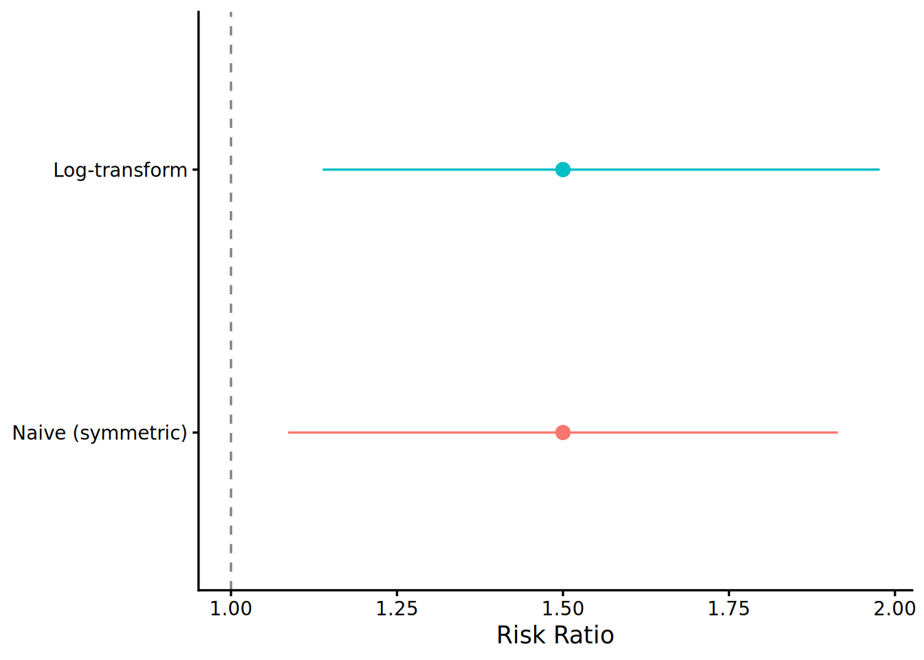
\[\text{95\% CI for } RR: \quad (e^{0.12959}, \; e^{0.68133}) = (1.138, \; 1.977)\]
The interval excludes \(1\), so the lift is statistically significant at the 5% level. The “relative lift” of 50% has a 95% CI of approximately (13.8%, 97.7%).
Naive symmetric CI (for comparison):
\[\text{Var}(\widehat{RR}) = 1.500^2 \times \left[\frac{1-0.210}{500 \times 0.210} + \frac{1-0.140}{500 \times 0.140}\right] = 2.25 \times (0.007524 + 0.012286) = 0.044573\]
\[SE_{naive} = \sqrt{0.044573} = 0.21112\]
\[\text{95\% CI}_{naive}: \quad 1.500 \pm 1.96 \times 0.21112 = (1.086, \; 1.914)\]
Both intervals exclude \(1\), but they differ in shape. The naive CI extends \(0.414\) in each direction. The log-transform CI extends \(0.362\) below and \(0.477\) above \(\widehat{RR}\), matching the right-skewed sampling distribution. The divergence grows with smaller \(n\) or larger \(\widehat{RR}\).
When the two methods diverge
The two intervals diverge most when the baseline rate \(p_0\) is low. Few positive responses in the control group make \(\hat{p}_0\) unstable, and the sampling distribution of \(\widehat{RR}\) is no longer well-approximated by a normal. The naive CI cannot reflect this; the log-transform CI can, because it is asymmetric by construction.
The log-transform CI is still an asymptotic method. It requires \(x_1\) and \(x_0\) to be large enough for the normal approximation to \(\log(\hat{p})\) to hold. When the expected positive count in the control group \(\mathbb{E}[x_0] = n \cdot p_0\) is small, the \(1/x_0\) term in the SE formula dominates, and the CI becomes wider than the stated confidence level implies.
R code
bls_rr_ci <- function(x1, n1, x0, n0, alpha = 0.05) {
  p1 <- x1 / n1
  p0 <- x0 / n0
  rr <- p1 / p0

  # Log-transform CI (delta method)
  se_log <- sqrt(1/x1 - 1/n1 + 1/x0 - 1/n0)
  z <- qnorm(1 - alpha / 2)
  ci_log <- exp(log(rr) + c(-1, 1) * z * se_log)

  # Naive symmetric CI
  var_rr <- rr^2 * ((1 - p1) / (n1 * p1) + (1 - p0) / (n0 * p0))
  ci_naive <- rr + c(-1, 1) * z * sqrt(var_rr)

  list(
    rr = rr,
    log_transform = ci_log,
    naive = ci_naive
  )
}

bls_rr_ci(105, 500, 70, 500)

# $rr
# [1] 1.5
#
# $log_transform
# [1] 1.138381 1.976491
#
# $naive
# [1] 1.086213 1.913787
SQL (BigQuery)
The same computation in SQL, no UDFs needed. If BLS results are already aggregated into cell counts per campaign, the CI is a single query:
with bls as (
  select
    study_id,
    x1,  -- exposed positive count
    n1,  -- exposed total
    x0,  -- control positive count
    n0   -- control total
  from bls_results
)

select
  study_id,
  (x1 / n1) / (x0 / n0) as rr,
  exp(
    ln((x1 / n1) / (x0 / n0))
    - 1.96 * sqrt(1/x1 - 1/n1 + 1/x0 - 1/n0)
  ) as ci_lower,
  exp(
    ln((x1 / n1) / (x0 / n0))
    + 1.96 * sqrt(1/x1 - 1/n1 + 1/x0 - 1/n0)
  ) as ci_upper
from bls
where x1 > 0 and x0 > 0  -- log undefined at zero