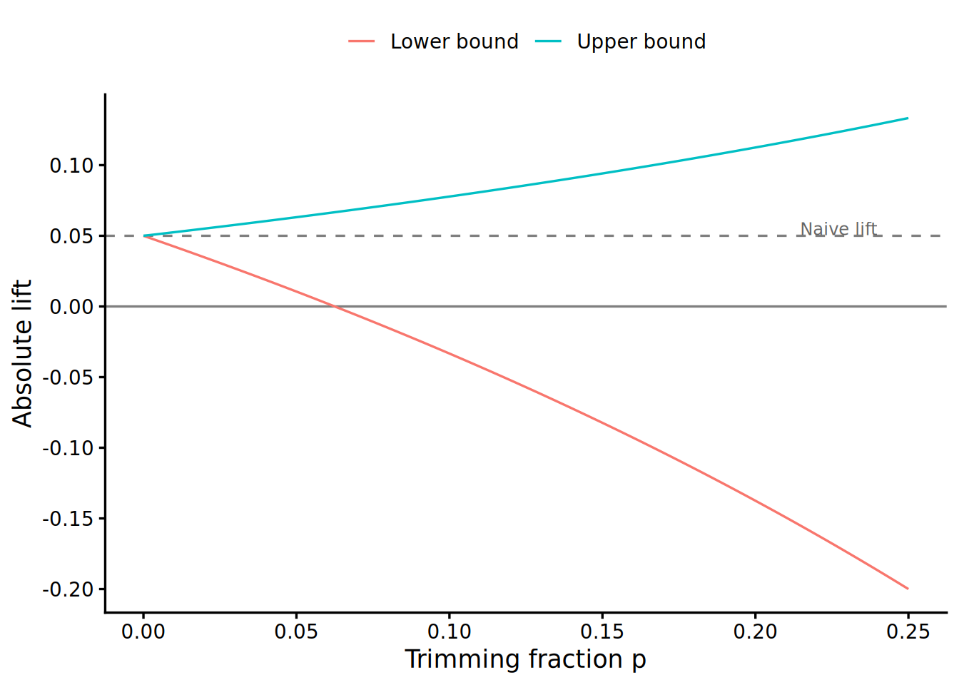
| \(p\) | Lower bound | Upper bound | Width |
|---|---|---|---|
| 0.020 | 0.035 | 0.055 | 0.020 |
| 0.050 | 0.011 | 0.063 | 0.053 |
| 0.080 | −0.015 | 0.072 | 0.087 |
| 0.100 | −0.033 | 0.078 | 0.111 |
| 0.150 | −0.082 | 0.094 | 0.176 |
| 0.200 | −0.138 | 0.112 | 0.250 |
Every Brand Lift Study (BLS) 2×2 table is built from survey respondents, not from everyone who was surveyed. If ad exposure changes who responds, the exposed and control groups are drawn from different subpopulations, and the risk ratio \(\widehat{RR}\) carries a selection bias that no CI method can remove.
This post introduces Lee bounds (Lee 2009) as a diagnostic for this problem. Lee bounds quantify how large the bias could be under a monotonicity assumption, without modeling the selection mechanism. The output is not a point estimate but a partially identified interval for the causal effect among always-responders: the subpopulation that would respond regardless of ad exposure. If the interval excludes zero, the lift is robust. If it spans zero, the naive \(\widehat{RR}\) may be an artifact of who showed up to answer the survey.
The selection problem in BLS
A BLS campaign delivers surveys to \(N_1\) exposed and \(N_0\) control individuals. Of these, \(n_1\) and \(n_0\) respond. The response rates are:
\[q_1 = \frac{n_1}{N_1}, \quad q_0 = \frac{n_0}{N_0}\]
The 2×2 table analyzed in the first post is built from respondents only. It records positive and negative responses among the \(n_1\) and \(n_0\) who answered, not among the \(N_1\) and \(N_0\) who were surveyed.
If \(q_1 = q_0\), the respondents in each group are a random subset of their respective populations, and comparing \(\hat{p}_1\) to \(\hat{p}_0\) estimates the causal effect of exposure. If \(q_1 \neq q_0\), the respondent subpopulations differ in composition. Some individuals respond only because they were exposed to the ad. The difference \(\hat{p}_1 - \hat{p}_0\) then conflates the effect of ad exposure on attitudes with the effect of ad exposure on who shows up in the data.
The CI methods from the previous posts handle sampling variability: the randomness in \(\hat{p}_1\) and \(\hat{p}_0\) given the respondent populations. Selection is a different problem: the non-randomness in who enters those populations in the first place.
Lee bounds: trimming under monotonicity
Setup and notation
Let \(Z \in \{0, 1\}\) denote treatment assignment (control vs. exposed), \(S \in \{0, 1\}\) denote whether the individual responds to the survey, and \(Y \in \{0, 1\}\) denote the outcome (negative vs. positive response). \(Y\) is observed only when \(S = 1\).
Each individual has potential outcomes \((S(0), S(1))\) for survey response and \((Y(0), Y(1))\) for the outcome. Treatment is randomly assigned (as in BLS), so \((S(z), Y(z))\) is independent of \(Z\).
Principal strata
The pair \((S(0), S(1))\) partitions the population into four strata:
| Stratum | \(S(0)\) | \(S(1)\) | Description |
|---|---|---|---|
| Always-responders | 1 | 1 | Respond regardless of exposure |
| Compliers | 0 | 1 | Respond only when exposed |
| Defiers | 1 | 0 | Respond only when not exposed |
| Never-responders | 0 | 0 | Do not respond regardless of exposure |
Two assumptions
Random assignment. \((S(z), Y(z)) \perp Z\). This holds by the BLS experimental design: exposed and control groups are assigned randomly.
Monotonicity. \(S(1) \geq S(0)\) for all individuals. Exposure does not cause anyone to stop responding. Under this assumption, the defier stratum is empty.
Monotonicity is not testable from the observed data. It is adopted as a structural assumption about the survey response process: seeing an ad may prompt someone to engage with a subsequent survey about the ad, but it does not suppress the response of someone who would have responded anyway. For BLS, this is an assumption rather than a fact: the reverse mechanism is constructible, since irritation with the ad could make someone decline a survey about it, and violations in that direction are outside what these bounds control. If the observed response rates show \(q_1 < q_0\), the assumption is applied in the reverse direction and the trimming moves to the control group. The formulas below assume \(q_1 \geq q_0\).
Strata proportions
Under random assignment, \(q_1 = P(S = 1 \mid Z = 1) = P(S(1) = 1)\) and \(q_0 = P(S = 1 \mid Z = 0) = P(S(0) = 1)\). Under monotonicity:
\[P(\text{always-responder}) = P(S(0) = 1) = q_0\]
\[P(\text{complier}) = P(S(1) = 1) - P(S(0) = 1) = q_1 - q_0\]
\[P(\text{never-responder}) = 1 - P(S(1) = 1) = 1 - q_1\]
The trimming fraction
Among the exposed respondents (\(Z = 1, S = 1\)), the proportion who are compliers is:
\[p = \frac{P(\text{complier})}{P(S(1) = 1)} = \frac{q_1 - q_0}{q_1}\]
The remaining fraction \(1 - p = q_0 / q_1\) are always-responders. The control respondents (\(Z = 0, S = 1\)) are all always-responders under monotonicity, since \(S(0) = 1\) implies the individual is in the always-responder stratum.
The estimand is the average treatment effect among always-responders:
\[\tau_{AR} = E[Y(1) - Y(0) \mid \text{always-responder}]\]
\(E[Y(0) \mid \text{always-responder}]\) is directly identified: it equals \(E[Y \mid Z = 0, S = 1]\), estimated by \(\hat{p}_0\), because all control respondents are always-responders.
\(E[Y(1) \mid \text{always-responder}]\) is not identified. The observed \(E[Y \mid Z = 1, S = 1] = \hat{p}_1\) is a mixture of always-responders and compliers, and the compliers’ potential outcomes under exposure are unknown.
Bounds for binary outcomes
To bound \(E[Y(1) \mid \text{always-responder}]\), consider two extreme assumptions about the compliers:
Lower bound. Assume every complier has \(Y(1) = 1\). This attributes the maximum possible share of the observed positive rate to compliers, leaving the minimum for always-responders:
\[\hat{p}_1^{L} = \max\!\left(0, \;\frac{\hat{p}_1 - p}{1 - p}\right)\]
Upper bound. Assume every complier has \(Y(1) = 0\). The entire observed positive rate is attributed to always-responders:
\[\hat{p}_1^{U} = \min\!\left(1, \;\frac{\hat{p}_1}{1 - p}\right)\]
The Lee bounds on \(\tau_{AR}\) are:
\[\left[\hat{p}_1^{L} - \hat{p}_0, \quad \hat{p}_1^{U} - \hat{p}_0\right]\]
These bounds are sharp under the two assumptions (random assignment and monotonicity): no tighter bounds can be obtained without additional assumptions about the compliers.
When differential attrition vanishes
If \(q_1 = q_0\), then \(p = 0\), and \(\hat{p}_1^{L} = \hat{p}_1^{U} = \hat{p}_1\). The bounds collapse to the point estimate \(\hat{p}_1 - \hat{p}_0\), which is the naive estimator. The naive \(\widehat{RR}\) is then unbiased for the always-responder effect, and the CIs from the previous posts apply directly.
Worked example: two scenarios
Take \(\hat{p}_1 = 0.250\) and \(\hat{p}_0 = 0.200\), giving a naive absolute lift of \(0.050\) and \(\widehat{RR} = 1.250\). The same naive estimate leads to opposite diagnostic conclusions depending on the response rate gap.
Scenario A: large differential attrition (\(q_1 = 0.30\), \(q_0 = 0.25\)).
\[p = \frac{0.30 - 0.25}{0.30} = 0.1667\]
\[\hat{p}_1^{L} = \frac{0.250 - 0.1667}{1 - 0.1667} = \frac{0.0833}{0.8333} = 0.100\]
\[\hat{p}_1^{U} = \frac{0.250}{0.8333} = 0.300\]
| Quantity | Value |
|---|---|
| Trimming fraction \(p\) | \(0.167\) |
| \(\hat{p}_1^{L}\) (always-responders) | \(0.100\) |
| \(\hat{p}_1^{U}\) (always-responders) | \(0.300\) |
| Bounds on absolute lift | \((-0.100,\; 0.100)\) |
| Bounds on \(RR\) | \((0.500,\; 1.500)\) |
The lower bound on absolute lift is \(-0.100\), and the lower bound on \(RR\) is \(0.500\). Both span the null. A 5-percentage-point gap in response rates is enough to explain away the entire observed lift of 5%. The positive rate in the exposed group could partly reflect compliers who are disproportionately likely to respond positively, not a genuine ad effect on always-responders.
Scenario B: small differential attrition (\(q_1 = 0.26\), \(q_0 = 0.25\)).
\[p = \frac{0.26 - 0.25}{0.26} = 0.0385\]
\[\hat{p}_1^{L} = \frac{0.250 - 0.0385}{1 - 0.0385} = \frac{0.2115}{0.9615} = 0.220\]
\[\hat{p}_1^{U} = \frac{0.250}{0.9615} = 0.260\]
| Quantity | Value |
|---|---|
| Trimming fraction \(p\) | \(0.038\) |
| \(\hat{p}_1^{L}\) (always-responders) | \(0.220\) |
| \(\hat{p}_1^{U}\) (always-responders) | \(0.260\) |
| Bounds on absolute lift | \((0.020,\; 0.060)\) |
| Bounds on \(RR\) | \((1.100,\; 1.300)\) |
The lower bound on absolute lift is \(0.020\): positive. The lower bound on \(RR\) is \(1.100\): above \(1\). The lift is robust. Even under the worst-case assumption about compliers, the always-responder effect remains positive.
Both scenarios share the same naive estimates. The diagnostic conclusion hinges entirely on the response rate gap \(q_1 - q_0\), a quantity not present in the standard BLS 2×2 table.
Binary outcomes reduce resolution
For binary outcomes, the width of the Lee bounds on \(E[Y(1) \mid \text{always-responder}]\) has a closed form. When both bounds are interior (strictly between 0 and 1):
\[\hat{p}_1^{U} - \hat{p}_1^{L} = \frac{\hat{p}_1}{1 - p} - \frac{\hat{p}_1 - p}{1 - p} = \frac{p}{1 - p}\]
The width depends only on the trimming fraction \(p\). It does not depend on \(\hat{p}_1\). The width of the bounds on \(\tau_{AR}\) is the same, since \(\hat{p}_0\) cancels.
At \(p = 0.10\), the width is \(0.111\), more than twice the naive absolute lift of \(0.050\). The bounds cross zero at \(p \approx 0.063\), corresponding to a response rate ratio of \(q_1 / q_0 \approx 1.07\).
The crossing point has a closed form. The lower bound on absolute lift is negative when:
\[\frac{\hat{p}_1 - p}{1 - p} < \hat{p}_0 \quad \Longleftrightarrow \quad p > \frac{\hat{p}_1 - \hat{p}_0}{1 - \hat{p}_0}\]
For \(\hat{p}_1 = 0.250\), \(\hat{p}_0 = 0.200\): the critical trimming fraction is \(p^* = \frac{0.050}{0.800} = 0.0625\).
This low threshold is a consequence of the binary outcome. Trimming operates by removing entire positive or negative responses. Each unit of trimming fraction shifts \(\hat{p}_1^L\) downward by a full step. With continuous outcomes, trimming removes only tail observations, and the conditional mean shifts more gradually. For BLS, where outcomes are always binary and typical lifts are in the range \(\hat{p}_1 - \hat{p}_0 \in [0.02, 0.05]\), even modest differential attrition can push the lower bound below zero.
When Lee bounds add value
Lee bounds are a sensitivity analysis for selection bias, not a replacement for \(\widehat{RR}\). They answer “could the effect be zero despite what the naive estimate says?” rather than “what is the effect?” Making them a permanent pipeline component is hard to justify. The computation is trivial, but the conceptual overhead of reporting partially identified intervals for every study is not.
The real value is as a one-time validation. Accumulate \(q_1 - q_0\) across a set of studies. If the distribution is tightly centered around zero, differential attrition is not a systematic concern, and the naive \(\widehat{RR}\) with its delta method CI can be trusted. If specific campaign types show elevated \(q_1 - q_0\), Lee bounds become a targeted diagnostic for those segments.
Running this validation requires survey delivery counts \(N_1\) and \(N_0\) alongside response counts \(n_1\) and \(n_0\). If the pipeline stores only the 2×2 table of respondents, the response rate gap cannot be computed after the fact.
R code
bls_lee_bounds <- function(q1, q0, p1_hat, p0_hat) {
  # Formulas assume trimming on the exposed group
  stopifnot(q1 >= q0)

  # Trimming fraction
  p <- (q1 - q0) / q1

  # Bounds on E[Y(1) | always-responder]
  p1_lower <- max(0, (p1_hat - p) / (1 - p))
  p1_upper <- min(1, p1_hat / (1 - p))

  # Bounds on treatment effect (absolute lift scale)
  tau_lower <- p1_lower - p0_hat
  tau_upper <- p1_upper - p0_hat

  # Bounds on RR scale
  rr_lower <- p1_lower / p0_hat
  rr_upper <- p1_upper / p0_hat

  list(
    p = p,
    p1_bounds = c(p1_lower, p1_upper),
    lift_bounds = c(tau_lower, tau_upper),
    rr_bounds = c(rr_lower, rr_upper)
  )
}

# From raw counts:
# N1, N0 = survey delivery counts
# n1, n0 = respondent counts
# x1, x0 = positive response counts
bls_lee_bounds_counts <- function(N1, N0, n1, n0, x1, x0) {
  q1 <- n1 / N1
  q0 <- n0 / N0
  p1_hat <- x1 / n1
  p0_hat <- x0 / n0
  bls_lee_bounds(q1, q0, p1_hat, p0_hat)
}

# Scenario A: large differential attrition
bls_lee_bounds(q1 = 0.30, q0 = 0.25, p1_hat = 0.250, p0_hat = 0.200)

# $p
# [1] 0.1666667
#
# $p1_bounds
# [1] 0.1 0.3
#
# $lift_bounds
# [1] -0.1  0.1
#
# $rr_bounds
# [1] 0.5 1.5

# Scenario B: small differential attrition
bls_lee_bounds(q1 = 0.26, q0 = 0.25, p1_hat = 0.250, p0_hat = 0.200)

# $p
# [1] 0.03846154
#
# $p1_bounds
# [1] 0.22 0.26
#
# $lift_bounds
# [1] 0.02 0.06
#
# $rr_bounds
# [1] 1.1 1.3

# Critical trimming fraction (bounds cross zero)
bls_critical_p <- function(p1_hat, p0_hat) {
  (p1_hat - p0_hat) / (1 - p0_hat)
}

bls_critical_p(0.250, 0.200)
# [1] 0.0625
For individual-level data \((Z_i, S_i, Y_i)\), the leebounds package computes Lee bounds with standard errors.