The previous post showed that the log-transform delta method CI for \(RR\) achieves its nominal 95% coverage when the expected number of positive control responses \(\mathbb{E}[x_0] = n \cdot p_0\) is 20 or more. Below that, the delta method becomes conservative: the \(\frac{1}{x_0}\) term in the SE formula inflates the interval beyond what the stated confidence level implies. The bootstrap percentile CI, which does not depend on the Taylor approximation, maintained near-nominal coverage across the full range.
If the bootstrap works everywhere, why not use it for everything? The bootstrap is not closed-form: it requires a simulation loop for each study, which rules out SQL implementation and adds computational cost in batch pipelines. It also does not produce a closed-form variance formula, which is needed for sample size calculations and meta-analytic weighting. This post introduces a third method, Fieller’s confidence interval (Fieller 1954), that removes the Taylor approximation while remaining closed-form and SQL-compatible.
Throughout, \(n_1 = n_0 = n\).
Three methods
Before deriving Fieller’s CI, it is worth comparing what each method provides. The following table summarizes the three methods covered in this series.
| Delta method | Fieller | Bootstrap | |
|---|---|---|---|
| Approximation layers | CLT + Taylor | CLT only | None (resampling) |
| Output | CI + closed-form variance formula | CI only | CI + variance estimate |
| SQL implementation | Yes | Yes | No (simulation loop) |
| Computational cost | \(O(1)\) per study | \(O(1)\) per study | \(O(B)\) per study |
| Small \(\mathbb{E}[x_0]\) coverage | Overcoverage | Near nominal | Near nominal |
| Insufficient data signal | None (always returns a finite CI) | Returns unbounded CI | None (always returns a finite CI) |
| Closed-form variance for downstream use | Yes | No | No |
The key differentiator is the closed-form variance formula. The first post derived \(\text{Var}(\log(\widehat{RR})) = \frac{1}{x_1} - \frac{1}{n_1} + \frac{1}{x_0} - \frac{1}{n_0}\), and the second post inverted it to solve for \(n_{\min}\). Meta-analysis weights each study by \(w_k = 1/\text{Var}(\log(\widehat{RR}_k))\). Only the delta method provides this formula as an algebraic expression in terms of cell counts; the bootstrap can estimate a variance numerically but cannot express it as a function of \(n\) to invert, and Fieller returns no variance at all. For a broader treatment of confidence intervals for ratios, including the geometric interpretation of Fieller’s theorem, see Franz (2007). The three methods are complementary. When \(\mathbb{E}[x_0] \geq 20\), all three produce nearly identical CIs and the delta method suffices for all purposes. The choice matters only below that threshold.
Fieller’s theorem
The delta method CI is built by approximating \(\text{Var}(\widehat{RR})\) via Taylor expansion and then constructing a Wald interval. Fieller’s approach is different: instead of approximating the variance of the ratio, it inverts a hypothesis test for each candidate value of \(RR\).
The CI is defined as the set of \(\theta\) values that are not rejected by the test \(H_0: RR = \theta\):
\[\text{CI} = \bigl\{\theta : H_0\!: RR = \theta \text{ is not rejected at level } \alpha \bigr\}\]
Under \(H_0\), \(p_1 = \theta \, p_0\), so \(\hat{p}_1 - \theta \hat{p}_0\) has mean zero. Since \(\hat{p}_1\) and \(\hat{p}_0\) are independent (the same assumption used throughout this series), the variance of the difference is additive:
\[\text{Var}(\hat{p}_1 - \theta \hat{p}_0) = \text{Var}(\hat{p}_1) + \theta^2 \, \text{Var}(\hat{p}_0)\]
Substituting the plug-in variance estimates \(V_1 = \frac{\hat{p}_1(1-\hat{p}_1)}{n}\) and \(V_0 = \frac{\hat{p}_0(1-\hat{p}_0)}{n}\), the test statistic is:
\[T(\theta) = \frac{(\hat{p}_1 - \theta \hat{p}_0)^2}{V_1 + \theta^2 V_0}\]
\(T(\theta)\) is compared to \(z^2 = z_{1-\alpha/2}^2\). The CI consists of all \(\theta\) satisfying \(T(\theta) \leq z^2\), which rearranges to:
\[(\hat{p}_1 - \theta \hat{p}_0)^2 \leq z^2(V_1 + \theta^2 V_0)\]
Expanding the left side and collecting terms in \(\theta\):
\[\hat{p}_1^2 - 2\theta \hat{p}_1 \hat{p}_0 + \theta^2 \hat{p}_0^2 \leq z^2 V_1 + z^2 \theta^2 V_0\]
\[\theta^2(\hat{p}_0^2 - z^2 V_0) - 2\theta \hat{p}_1 \hat{p}_0 + (\hat{p}_1^2 - z^2 V_1) \leq 0\]
This is a quadratic inequality \(a\theta^2 - 2b\theta + c \leq 0\) with coefficients:
\[a = \hat{p}_0^2 - z^2 V_0, \quad b = \hat{p}_1 \hat{p}_0, \quad c = \hat{p}_1^2 - z^2 V_1\]
When \(a > 0\) and the discriminant \(D = b^2 - ac\) is positive, the quadratic has two real roots and the CI is the closed interval between them:
\[\text{CI}_{\text{Fieller}} = \left[\frac{b - \sqrt{D}}{a}, \; \frac{b + \sqrt{D}}{a}\right]\]
No Taylor expansion appears anywhere in this derivation. The only approximation is the CLT: \(\hat{p}_1\) and \(\hat{p}_0\) are treated as normally distributed, same as in the delta method. Instead of linearizing the ratio, Fieller solves a quadratic equation.
Bounded condition
The CI is bounded when \(a > 0\). (In principle, \(D \geq 0\) is also required, but this holds whenever both sample proportions are positive.) Expanding:
\[\hat{p}_0^2 > z^2 \frac{\hat{p}_0(1 - \hat{p}_0)}{n} \quad \Longleftrightarrow \quad n \hat{p}_0 > z^2(1 - \hat{p}_0) \quad \Longleftrightarrow \quad x_0 > z^2(1 - \hat{p}_0)\]
For a 95% CI (\(z^2 = 3.84\)) and small \(\hat{p}_0\), this reduces to approximately \(x_0 \geq 4\).
When \(a \leq 0\), the control group has too few positive responses to distinguish its rate from zero. The CI becomes unbounded because the data cannot pin down \(RR\). Avoid reporting a CI; flag the study as underpowered.
The delta method does not signal this problem. It returns a finite CI for any \(x_0 \geq 1\), regardless of whether the data support it. The previous post showed the consequence: at \(\mathbb{E}[x_0] = 2\), delta method coverage exceeds 99%, meaning the interval is far wider than a 95% CI should be.
Asymptotic equivalence to the delta method
As \(n\) grows, \(V_0\) and \(V_1\) shrink to zero, so \(a \to \hat{p}_0^2\) and \(c \to \hat{p}_1^2\). The center of the Fieller CI converges to \(b/a \to \hat{p}_1/\hat{p}_0 = \widehat{RR}\).
For the width, expand the discriminant:
\[D = b^2 - ac = \hat{p}_1^2 \hat{p}_0^2 - (\hat{p}_0^2 - z^2 V_0)(\hat{p}_1^2 - z^2 V_1) = z^2(\hat{p}_0^2 V_1 + \hat{p}_1^2 V_0) - z^4 V_0 V_1\]
The \(z^4 V_0 V_1\) term is \(O(n^{-2})\). Dropping it and substituting into the CI bounds:
\[\frac{b \pm \sqrt{D}}{a} \approx \frac{\hat{p}_1 \hat{p}_0 \pm z\sqrt{\hat{p}_0^2 V_1 + \hat{p}_1^2 V_0}}{\hat{p}_0^2} = \widehat{RR} \pm \frac{z}{\hat{p}_0^2}\sqrt{\hat{p}_0^2 V_1 + \hat{p}_1^2 V_0}\]
Substituting \(V_1 = \hat{p}_1(1-\hat{p}_1)/n\) and \(V_0 = \hat{p}_0(1-\hat{p}_0)/n\) and simplifying:
\[= \widehat{RR} \pm z\sqrt{\widehat{RR}^2 \left[\frac{1-\hat{p}_1}{n\hat{p}_1} + \frac{1-\hat{p}_0}{n\hat{p}_0}\right]}\]
The expression under the square root is \(\text{Var}(\widehat{RR})\) from the first post. For large \(n\), Fieller’s CI coincides with the naive symmetric delta method CI. The log-transform CI from that post also converges to the same interval, since both are first-order approximations. The practical implication: when \(\mathbb{E}[x_0]\) is large enough, Fieller offers no advantage over the delta method.
Worked example
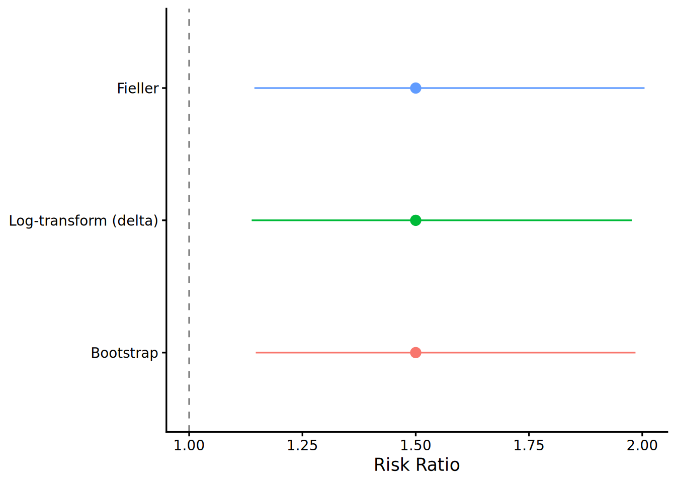
The same data as the first post:
| Positive | Negative | Total | |
|---|---|---|---|
| Exposed | 105 | 395 | 500 |
| Control | 70 | 430 | 500 |
\[\hat{p}_1 = 0.210, \quad \hat{p}_0 = 0.140, \quad \widehat{RR} = 1.500\]
Compute the plug-in variances:
\[V_1 = \frac{0.210 \times 0.790}{500} = 0.0003318, \quad V_0 = \frac{0.140 \times 0.860}{500} = 0.0002408\]
With \(z^2 = 1.96^2 = 3.8416\):
\[a = 0.140^2 - 3.8416 \times 0.0002408 = 0.019600 - 0.000925 = 0.018675\]
\[b = 0.210 \times 0.140 = 0.029400\]
\[c = 0.210^2 - 3.8416 \times 0.0003318 = 0.044100 - 0.001275 = 0.042825\]
Bounded condition: \(x_0 = 70 > z^2(1 - \hat{p}_0) = 3.8416 \times 0.860 = 3.304\). The CI is bounded.
\[D = 0.029400^2 - 0.018675 \times 0.042825 = 0.00086436 - 0.00079972 = 0.00006464\]
\[\sqrt{D} = 0.008040\]
\[\text{CI}_{\text{Fieller}}: \quad \left(\frac{0.029400 - 0.008040}{0.018675}, \; \frac{0.029400 + 0.008040}{0.018675}\right) = (1.144, \; 2.005)\]
For comparison, the log-transform delta method CI from the first post is \((1.138, \; 1.977)\). The Fieller CI is slightly wider, especially on the upper tail. At \(\mathbb{E}[x_0] = 70\), the difference is small. Both intervals exclude \(1\).
Coverage simulation
Design
The simulation grid is identical to the previous post: four baseline rates, three sample sizes, and one confirmation condition. Fieller’s CI is added as a third method evaluated on the same replicated datasets. Replications where \(x_1 = 0\) or \(x_0 = 0\) are skipped for all methods.
| Parameter | Values |
|---|---|
| \(RR\) | \(1.20\) (primary), \(1.50\) (confirmation) |
| \(p_0\) | \(0.02, \; 0.05, \; 0.10, \; 0.20\) |
| \(n \; (= n_1 = n_0)\) | \(100, \; 500, \; 2{,}000\) |
| Replications | \(K = 10{,}000\) |
| Confidence level | \(95\%\) |
For Fieller, an unbounded CI (where \(a \leq 0\)) is counted as covering the true \(RR\), since the confidence set includes all real values. The rate of unbounded CIs is reported separately.
Results
| \(p_0\) | \(n\) | \(RR\) | \(\mathbb{E}[x_0]\) | Delta method | Fieller | Bootstrap | Fieller unbounded |
|---|---|---|---|---|---|---|---|
| 0.02 | 100 | 1.20 | 2 | 99.9% | 99.7% | 99.3% | 84.8% |
| 0.05 | 100 | 1.20 | 5 | 97.7% | 98.0% | 95.4% | 24.8% |
| 0.05 | 100 | 1.50 | 5 | 97.6% | 98.1% | 95.6% | 25.1% |
| 0.02 | 500 | 1.20 | 10 | 95.5% | 95.1% | 94.4% | 1.0% |
| 0.10 | 100 | 1.20 | 10 | 96.1% | 95.0% | 94.4% | 0.9% |
| 0.20 | 100 | 1.20 | 20 | 95.2% | 94.3% | 94.6% | 0.0% |
| 0.05 | 500 | 1.20 | 25 | 95.5% | 95.1% | 95.0% | 0.0% |
| 0.02 | 2,000 | 1.20 | 40 | 95.7% | 95.5% | 95.3% | 0.0% |
| 0.10 | 500 | 1.20 | 50 | 95.4% | 95.1% | 95.2% | 0.0% |
| 0.05 | 2,000 | 1.20 | 100 | 94.6% | 94.5% | 94.5% | 0.0% |
| 0.20 | 500 | 1.20 | 100 | 95.3% | 95.1% | 95.1% | 0.0% |
| 0.10 | 2,000 | 1.20 | 200 | 95.2% | 95.0% | 95.0% | 0.0% |
| 0.20 | 2,000 | 1.20 | 400 | 95.1% | 95.1% | 95.2% | 0.0% |
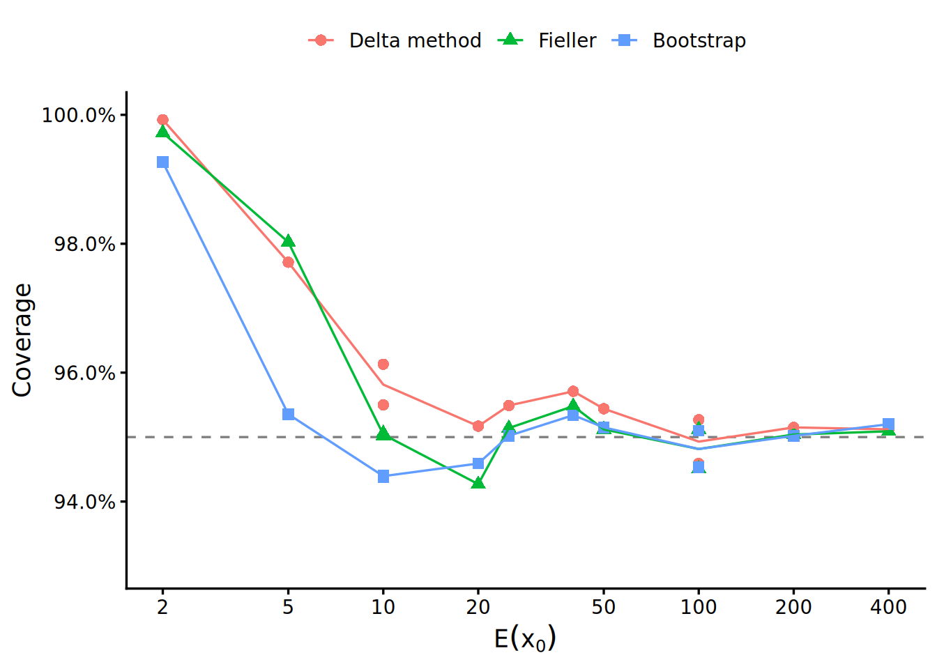
Figure 2 and Table 1 extend the picture from the previous post.
Large \(\mathbb{E}[x_0]\): all three methods agree. At \(\mathbb{E}[x_0] \geq 50\), all three land within about one percentage point of 95%. The choice of method has little practical effect.
Small \(\mathbb{E}[x_0]\): the picture splits. At \(\mathbb{E}[x_0] = 10\), where unbounded rates are around 1%, Fieller’s coverage is closer to 95% than the delta method’s. The improvement comes from removing the Taylor layer: Fieller does not inflate the SE through the \(\frac{1}{x_0}\) term because it does not compute an SE at all.
At \(\mathbb{E}[x_0] = 5\), Fieller’s coverage exceeds the delta method’s. This reflects the unbounded CIs, not better accuracy: 25% of Fieller CIs are unbounded, and counting them as covering inflates the unconditional coverage. The useful output here is not the coverage number but the unbounded rate itself, which flags that one in four studies at this expected count cannot produce a meaningful CI.
Very small \(\mathbb{E}[x_0]\): CLT limits all methods. At \(\mathbb{E}[x_0] = 2\), the normal approximation to \(\hat{p}_0\) itself is poor. Fieller returns an unbounded CI in 85% of replications, reflecting that the data cannot support a finite interval. The delta method’s 99.9% coverage at \(\mathbb{E}[x_0] = 2\) indicates an interval too wide to be informative, not reliable estimation.
When to use which
The following table maps \(\mathbb{E}[x_0]\) ranges to recommended methods, by use case.
| \(\mathbb{E}[x_0]\) | CI for a single study | Power / \(n_{\min}\) calculation | Meta-analytic weight | SQL batch pipeline |
|---|---|---|---|---|
| \(\geq 20\) | Delta method | Delta method | Delta method | Delta method |
| \(5\) to \(20\) | Fieller | Delta method | Delta method | Fieller |
| \(< 5\) | Avoid reporting | — | — | — |
In the \(5\) to \(20\) range, the CI and the variance formula serve different purposes. The Fieller CI is more accurate for reporting the uncertainty around \(\widehat{RR}\), but it does not produce a variance. The delta method variance formula \(\frac{1}{x_1} - \frac{1}{n_1} + \frac{1}{x_0} - \frac{1}{n_0}\) is still computable and still usable for power calculations and weighting, even though the CI derived from it overcovers. The CI precision issue does not invalidate the variance formula for these downstream purposes; it only means the CI endpoints constructed from that variance are too wide.
The bootstrap’s role is validation. It is the least assumption-dependent method and the natural benchmark for checking whether a closed-form CI is performing correctly. It is not suited for production CI computation due to SQL incompatibility and \(O(B)\) cost per study. For ad-hoc analysis of a single study or for auditing a pipeline, the bootstrap remains the right tool.
R code
bls_rr_ci <- function(x1, n1, x0, n0, alpha = 0.05) {
  p1 <- x1 / n1
  p0 <- x0 / n0
  rr <- p1 / p0

  se_log <- sqrt(1/x1 - 1/n1 + 1/x0 - 1/n0)
  z <- qnorm(1 - alpha / 2)
  exp(log(rr) + c(-1, 1) * z * se_log)
}

bls_fieller_ci <- function(x1, n1, x0, n0, alpha = 0.05) {
  p1 <- x1 / n1
  p0 <- x0 / n0
  z2 <- qnorm(1 - alpha / 2)^2

  V1 <- p1 * (1 - p1) / n1
  V0 <- p0 * (1 - p0) / n0

  a  <- p0^2 - z2 * V0
  b  <- p1 * p0
  cc <- p1^2 - z2 * V1

  # Unbounded: control positive rate not distinguishable from zero
  if (a <= 0) return(c(NA, NA))

  D <- b^2 - a * cc
  if (D < 0) return(c(NA, NA))

  c((b - sqrt(D)) / a, (b + sqrt(D)) / a)
}

bls_bootstrap_ci <- function(x1, n1, x0, n0, B = 10000, alpha = 0.05) {
  p1_hat <- x1 / n1
  p0_hat <- x0 / n0
  x1_star <- rbinom(B, n1, p1_hat)
  x0_star <- rbinom(B, n0, p0_hat)

  valid <- x0_star > 0 & x1_star > 0
  rr_star <- (x1_star[valid] / n1) / (x0_star[valid] / n0)
  quantile(rr_star, c(alpha / 2, 1 - alpha / 2))
}

bls_rr_ci(105, 500, 70, 500)
# [1] 1.138381 1.976491

bls_fieller_ci(105, 500, 70, 500)
# [1] 1.143826 2.004849

bls_bootstrap_ci(105, 500, 70, 500)
#     2.5%    97.5%
# 1.146667 1.984854
SQL (BigQuery)
Fieller’s CI requires the quadratic coefficients \(a\), \(b\), \(c\) and the discriminant \(D\). When \(a \leq 0\) or \(D < 0\), the query returns NULL to signal an unbounded or empty interval.
with bls as (
  select
    study_id,
    x1,  -- exposed positive count
    n1,  -- exposed total
    x0,  -- control positive count
    n0   -- control total
  from bls_results
  where x1 > 0 and x0 > 0
),

props as (
  select
    study_id,
    x1, n1, x0, n0,
    x1 / n1 as p1,
    x0 / n0 as p0
  from bls
),

coefs as (
  select
    study_id,
    p1, p0,
    p1 / p0 as rr,
    pow(p0, 2) - 3.8416 * p0 * (1 - p0) / n0 as a,
    p1 * p0 as b,
    pow(p1, 2) - 3.8416 * p1 * (1 - p1) / n1 as c
  from props
),

disc as (
  select
    *,
    pow(b, 2) - a * c as d
  from coefs
)

select
  study_id,
  rr,
  case
    when a <= 0 or d < 0 then null
    else (b - sqrt(d)) / a
  end as ci_lower,
  case
    when a <= 0 or d < 0 then null
    else (b + sqrt(d)) / a
  end as ci_upper
from disc