| \(p_0\) | \(n\) | \(RR\) | \(\mathbb{E}[x_0]\) | Delta method | Bootstrap |
|---|---|---|---|---|---|
| 0.02 | 100 | 1.20 | 2 | 99.9% | 99.3% |
| 0.05 | 100 | 1.20 | 5 | 97.7% | 95.4% |
| 0.05 | 100 | 1.50 | 5 | 97.6% | 95.6% |
| 0.02 | 500 | 1.20 | 10 | 95.5% | 94.4% |
| 0.10 | 100 | 1.20 | 10 | 96.1% | 94.4% |
| 0.20 | 100 | 1.20 | 20 | 95.2% | 94.6% |
| 0.05 | 500 | 1.20 | 25 | 95.5% | 95.0% |
| 0.02 | 2,000 | 1.20 | 40 | 95.7% | 95.3% |
| 0.10 | 500 | 1.20 | 50 | 95.4% | 95.2% |
| 0.05 | 2,000 | 1.20 | 100 | 94.6% | 94.5% |
| 0.20 | 500 | 1.20 | 100 | 95.3% | 95.1% |
| 0.10 | 2,000 | 1.20 | 200 | 95.2% | 95.0% |
| 0.20 | 2,000 | 1.20 | 400 | 95.1% | 95.2% |
The previous post derived a log-transform delta method CI for the risk ratio \(RR = \frac{p_1}{p_0}\):
\[\left( \widehat{RR} \cdot e^{-z_{1-\alpha/2} \cdot SE}, \quad \widehat{RR} \cdot e^{+z_{1-\alpha/2} \cdot SE} \right)\]
where \(SE = \sqrt{\frac{1}{x_1} - \frac{1}{n_1} + \frac{1}{x_0} - \frac{1}{n_0}}\).
It is closed-form, computable in SQL, and always positive. But it is based on a first-order Taylor approximation. Brand Lift Study (BLS) campaigns run at finite sample sizes, and the baseline rate \(p_0\) can be low. How does the interval actually perform?
This post answers that question by simulation. A bootstrap percentile CI serves as the comparison method: it does not depend on the normal approximation that the delta method requires. Both are evaluated by coverage, the proportion of simulated datasets where the CI contains the true \(RR\).
The short version: when the expected number of positive control responses \(\mathbb{E}[x_0] = n \cdot p_0\) is 20 or more, the delta method CI achieves its nominal 95% coverage. Below that, it becomes conservative, producing intervals wider than the stated level implies. The second half of the post derives the minimum per-group sample size \(n_{\min}\) required to detect a given lift with a target power.
Throughout, \(n_1 = n_0 = n\), for simplicity.
Bootstrap percentile CI for RR
The bootstrap percentile CI does not require the normal approximation underlying the delta method. It is a parametric bootstrap: resample from the estimated binomial distributions and take quantiles.
Given observed counts \((x_1, n, x_0, n)\):
- Compute \(\hat{p}_1 = \frac{x_1}{n}\) and \(\hat{p}_0 = \frac{x_0}{n}\).
- For \(b = 1, \dots, B\): draw \(x_1^* \sim \text{Binomial}(n, \hat{p}_1)\) and \(x_0^* \sim \text{Binomial}(n, \hat{p}_0)\) independently. If \(x_0^* = 0\), discard the replicate (\(\widehat{RR}^*\) is undefined). Otherwise compute \(\widehat{RR}^*_b = (x_1^*/n) / (x_0^*/n)\).
- The \((1-\alpha)\) CI is \(\left( \widehat{RR}^*_{(\alpha/2)}, \; \widehat{RR}^*_{(1-\alpha/2)} \right)\).
Coverage simulation
Why fix RR?
The simulation varies \(p_0\) and \(n\) but holds \(RR\) fixed. Here is why.
\(\log(\widehat{RR}) = \log(\hat{p}_1) - \log(\hat{p}_0)\), and the two terms are independent. The normal approximation to their difference is only as good as the worse of the two individual approximations.
The delta method approximation to \(\log(\hat{p})\) depends on the expected count \(np = \mathbb{E}[x]\). Large \(np\) means \(\hat{p}\) is approximately normal and \(\log(\hat{p})\) inherits that normality. Small \(np\) means \(\hat{p}\) is discrete and right-skewed, and the approximation breaks down.
With \(n_1 = n_0 = n\) and \(RR > 1\), \(p_1 = RR \cdot p_0 > p_0\), so \(np_1 > np_0\) always. The exposed group always has more expected positive responses than control. The approximation to \(\log(\hat{p}_0)\) is always the weaker link.
The accuracy of \(\log(\hat{p}_0)\)’s approximation depends on \(np_0\) alone. \(RR\) affects \(p_1\) but not \(p_0\). Changing \(RR\) does not shift the threshold where the delta method starts to deviate.
The main simulation uses \(RR = 1.20\), a moderate lift typical of BLS campaigns (I think). One confirmation condition at \(RR = 1.50\) checks the \(RR\)-independence numerically.
Design
The key quantity is \(\mathbb{E}[x_0] = n \cdot p_0\). The grid varies both \(p_0\) and \(n\) to generate a range of \(\mathbb{E}[x_0]\) values.
| Parameter | Values |
|---|---|
| \(RR\) | \(1.20\) (primary), \(1.50\) (confirmation) |
| \(p_0\) | \(0.02, \; 0.05, \; 0.10, \; 0.20\) |
| \(n \; (= n_1 = n_0)\) | \(100, \; 500, \; 2{,}000\) |
| Replications | \(K = 10{,}000\) |
| Confidence level | \(95\%\) |
Four \(p_0\) values span BLS baseline rates at half-log spacing. Three \(n\) values produce 12 conditions with 10 unique \(\mathbb{E}[x_0]\) from 2 to 400:
| \(n = 100\) | \(n = 500\) | \(n = 2{,}000\) | |
|---|---|---|---|
| \(p_0 = 0.02\) | 2 | 10 | 40 |
| \(p_0 = 0.05\) | 5 | 25 | 100 |
| \(p_0 = 0.10\) | 10 | 50 | 200 |
| \(p_0 = 0.20\) | 20 | 100 | 400 |
Two pairs share the same \(\mathbb{E}[x_0]\): \(\mathbb{E}[x_0] = 10\) from \((0.02,\, 500)\) and \((0.10,\, 100)\); \(\mathbb{E}[x_0] = 100\) from \((0.05,\, 2{,}000)\) and \((0.20,\, 500)\). These test whether \(\mathbb{E}[x_0]\) alone determines coverage.
Each replication draws \(x_1 \sim \text{Binomial}(n, p_1)\) and \(x_0 \sim \text{Binomial}(n, p_0)\) from the true parameters, computes both CIs, and records whether each contains the true \(RR\). Replications where either count is zero are skipped.
Results
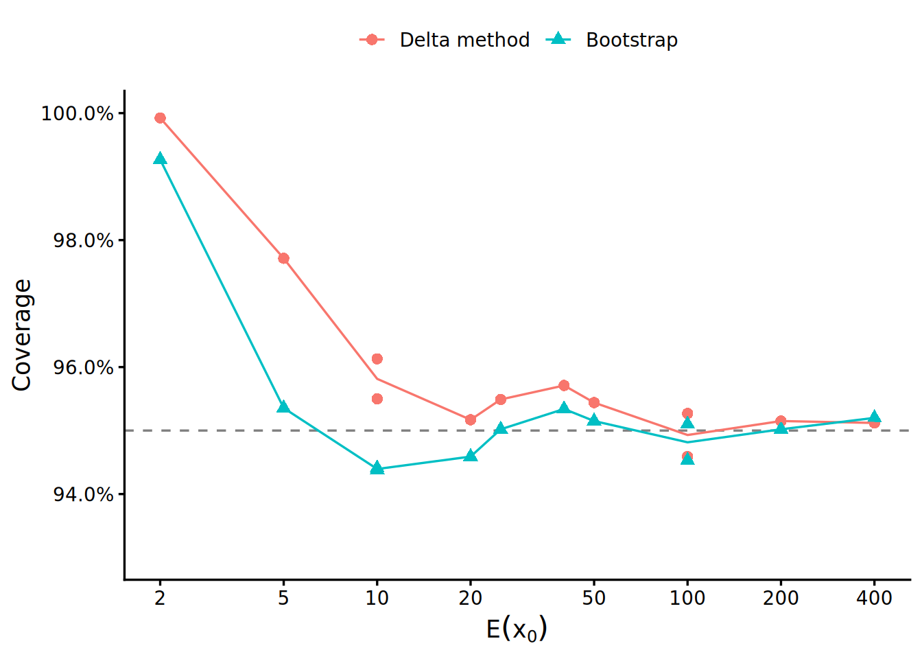
Figure 1 and Table 1 tell a clear story.
Large \(\mathbb{E}[x_0]\): the methods agree. At \(\mathbb{E}[x_0] \geq 50\), both methods land within about one percentage point of 95%. The delta method CI works as advertised.
Small \(\mathbb{E}[x_0]\): the delta method overcovers. Below \(\mathbb{E}[x_0] \approx 20\), coverage climbs above 95% for both methods, with the delta method rising faster. At \(\mathbb{E}[x_0] = 5\), delta method coverage is around 97.5%. At \(\mathbb{E}[x_0] = 2\), it exceeds 99%.
The mechanism is the \(\frac{1}{x_0}\) term in \(SE = \sqrt{\frac{1}{x_1} - \frac{1}{n_1} + \frac{1}{x_0} - \frac{1}{n_0}}\). When \(x_0\) is 1, 2, or 3, this term dominates and inflates the SE, producing intervals far wider than the stated level implies. The CI is still valid (it covers at least 95% of the time) but conservative: the stated 95% does not reflect the actual coverage.
RR-independence confirmed. At \(\mathbb{E}[x_0] = 5\), the \(RR = 1.50\) confirmation condition produces coverage nearly identical to \(RR = 1.20\), as predicted.
\(\mathbb{E}[x_0]\) sufficiency. The duplicate pairs (\(\mathbb{E}[x_0] = 10\) and \(100\), each from two different \((p_0, n)\) combinations) show coverage differences under one percentage point. \(\mathbb{E}[x_0]\) is the primary driver.
Minimum sample size
The delta method CI is reliable when \(\mathbb{E}[x_0]\) is large enough. The practical question: how many respondents per group does a study need to detect a given lift?
From CI to power
A lift is detected when the CI lower bound exceeds 1. On the log scale:
\[\log(\widehat{RR}) - z_{1-\alpha/2} \cdot SE > 0\]
Under the true \(RR\), \(\log(\widehat{RR}) \sim N(\log(RR), \; SE^2)\) approximately. Power is the probability of detection:
\[\text{Power} = P\!\left(\log(\widehat{RR}) > z_{1-\alpha/2} \cdot SE\right) = \Phi\!\left(\frac{\log(RR)}{SE} - z_{1-\alpha/2}\right)\]
Setting power to \(1 - \beta\) and solving:
\[\frac{\log(RR)}{SE} = z_{1-\alpha/2} + z_{1-\beta}\]
Derivation of \(n_{\min}\)
Set \(n_1 = n_0 = n\). From \(\log(RR) = (z_{1-\alpha/2} + z_{1-\beta}) \cdot SE\) and \(SE^2 = \frac{1-p_1}{n\,p_1} + \frac{1-p_0}{n\,p_0}\), solve for \(n\):
\[n_{\min} = \left\lceil \frac{(z_{1-\alpha/2} + z_{1-\beta})^2}{[\log(RR)]^2}\left[\frac{1-p_1}{p_1} + \frac{1-p_0}{p_0}\right] \right\rceil\]
Since \(p_1 = RR \cdot p_0\), the formula takes four inputs: \(p_0\), \(RR\), \(\alpha\), and power (\(1-\beta\)).
Worked example
Planning inputs from historical study norms: \(p_0 = 0.10\), \(RR = 1.20\) (20% relative lift). Target: 80% power at \(\alpha = 0.05\). Then \(p_1 = 0.12\), \(z_{0.975} = 1.96\), \(z_{0.80} = 0.842\), and:
\[n_{\min} = \left\lceil \frac{(1.96 + 0.842)^2}{[\log(1.20)]^2}\left[\frac{1-0.12}{0.12} + \frac{1-0.10}{0.10}\right] \right\rceil = \left\lceil \frac{7.849}{0.03324} \times 16.333 \right\rceil = \left\lceil 236.1 \times 16.333 \right\rceil = 3{,}857\]
At 80% power, the study needs approximately 3,900 respondents per group to detect a 20% relative lift.
\(p_0\) and \(RR\) are planning assumptions, typically from historical norms; if the actual values deviate, the realized power will differ.
\(n_{\min}\) reference table
| \(p_0\) | \(RR\) | \(n_{\min}\) |
|---|---|---|
| 0.05 | 1.10 | 31,263 |
| 0.05 | 1.20 | 8,186 |
| 0.05 | 1.50 | 1,496 |
| 0.10 | 1.10 | 14,768 |
| 0.10 | 1.20 | 3,857 |
| 0.10 | 1.50 | 701 |
| 0.20 | 1.10 | 6,520 |
| 0.20 | 1.20 | 1,693 |
| 0.20 | 1.50 | 303 |
R code
bls_rr_ci <- function(x1, n1, x0, n0, alpha = 0.05) {
  p1 <- x1 / n1
  p0 <- x0 / n0
  rr <- p1 / p0

  se_log <- sqrt(1/x1 - 1/n1 + 1/x0 - 1/n0)
  z <- qnorm(1 - alpha / 2)
  exp(log(rr) + c(-1, 1) * z * se_log)
}

bls_bootstrap_ci <- function(x1, n1, x0, n0, B = 10000, alpha = 0.05) {
  p1_hat <- x1 / n1
  p0_hat <- x0 / n0
  x1_star <- rbinom(B, n1, p1_hat)
  x0_star <- rbinom(B, n0, p0_hat)

  # Discard replicates where x0* = 0 (RR undefined)
  valid <- x0_star > 0 & x1_star > 0
  rr_star <- (x1_star[valid] / n1) / (x0_star[valid] / n0)
  quantile(rr_star, c(alpha / 2, 1 - alpha / 2))
}

bls_nmin <- function(p0, rr, alpha = 0.05, power = 0.80) {
  p1 <- rr * p0
  z_alpha <- qnorm(1 - alpha / 2)
  z_beta <- qnorm(power)
  ceiling(
    (z_alpha + z_beta)^2 / log(rr)^2
    * ((1 - p1) / p1 + (1 - p0) / p0)
  )
}

bls_rr_ci(105, 500, 70, 500)
# [1] 1.138381 1.976491

bls_bootstrap_ci(105, 500, 70, 500)
#     2.5%    97.5%
# 1.146667 1.984854

bls_nmin(p0 = 0.10, rr = 1.20)
# [1] 3857